Master VLOOKUP and XLOOKUP in Excel in 5 Steps

Master VLOOKUP and XLOOKUP in Excel in 5 Steps

🧰

Instant Toolkit

2 artifacts

📋
Step-by-Step Guide

1

Step 1: Understand VLOOKUP

Read the official Microsoft documentation on VLOOKUP.

Syntax

=VLOOKUP(lookup_value, table_array, col_index_num, [range_lookup])

  • lookup_value: Value to find in first column.
  • table_array: Range with lookup value in first column.
  • col_index_num: Column number to return (1-based).
  • range_lookup: FALSE for exact match (recommended), TRUE for approximate.

Example Setup

Create a table in Excel:

ABC
IDNamePrice
101Apple1.99
102Banana0.99

In D2: =VLOOKUP(101, A2:C3, 2, FALSE) → Returns "Apple".

Tips: Use absolute references like $A$2:$C$3. First column must contain lookup_value.

Why this step matters:
  • -Builds foundation for data retrieval in spreadsheets
  • -Essential for matching and pulling info from tables in daily tasks
30-45 minutes
Microsoft Excel, VLOOKUP Docs (support.microsoft.com), Notepad for notes
$0
Definition of Done
  • Explain VLOOKUP syntax in own words
  • Replicate basic example successfully
Common Mistakes to Avoid

Forgetting FALSE for exact match, getting wrong results

Always specify FALSE unless approximate match needed

Lookup value not in first column

Rearrange table or use INDEX/MATCH

Data types mismatch (text vs number)

Use VALUE() or TEXT() to convert

2

Following along, or just reading? 👀

Spin up a personalized “learn VLOOKUP and XLOOKUP” plan you can save, check off, and return to anytime — unlimited on the free trial.

Start free trial →
3
4
5